4.5. Temporal interpolation
Time-varying data as inputs into JULES are provided in two types - instantaneous states (e.g. air temperature, surface pressure, lai) or fluxes (e.g. radiation, precipitation). Because the data are on discrete timesteps, the value of an instantaneous variable applies at the timestamp (e.g. air temperature at 0800). However, values of the fluxes represent averages over the data timestep (e.g. 3-hour average rates). Different datasets supply the data as averages over the previous data timestep (backwards average) or the next data timestep (forwards average).
In order for the numerics to remain stable, it is recommended to run JULES with a model timestep of 1 hour or shorter. If the data timestep is longer than the model timestep, interpolation is required. How interpolation is performed for a particular variable depends on whether the variable is an instantaneous state or a flux.
4.5.1. Interpolation flags
When JULES needs to know what type of interpolation to use for a variable, the following flags are used.
iLinear interpolation from the data timestep to the model timestep.
For instantaneous data (e.g. air temperature, surface pressure), this is almost always the flag that should be used.
nb,ncandnfValues will be held constant with time for all model timesteps associated with a particular data timestep.
One of these flags should be used for flux variables that are discontinuous by nature, e.g. precipitation.
nbshould be used if the dataset uses backwards average values,nfshould be used if the data set uses forwards average values andncshould be used if the dataset uses centred average values (this is quite rare).b,candfData is interpolated using a simplified version of the Sheng and Zwiers (1998) [1] method that conserves the period means of the data.
One of these flags should be used for flux variables that are continuous in nature, e.g. radiation.
In order to ensure conservation of the average, these flags should be used only if the data period is an even multiple of the model timestep (i.e., if
data_period = 2 * n * timestep_len; n = 1, 2, 3, ...). The curve-fitting process tends to produce occasional values near turning points that fall outside the range of the input values.Similar to above,
bshould be used if the dataset uses backwards average values,fshould be used if the data set uses forwards average values andcshould be used if the dataset uses centred average values.
In order to perform interpolation, JULES may require input data for one or two data timesteps that fall before or after the times for the integration:
| Flag | Extra data timesteps required |
|---|---|
nf |
Only requires data that falls within the integration times |
i, nb, nc |
Requires one data timestep beyond the end of the integration |
nb |
Requires two data timesteps beyond the end of the integration |
nf |
Requires one data timestep before the start and one data timestep beyond the end of the integration |
nc |
Requires one data timestep before the start and two data timesteps beyond the end of the integration |
Also, note that for centred data (flags c and nc) the time of the data should be given as that at the start of the averaging period, rather than the centre, e.g. the 3-hour average over 06H to 09H, centred at 07:30H, should be treated as having timestamp 06H.
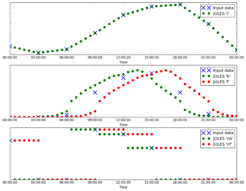
Examples of data interpolated with i, nb, nf, b and f, plotted against the data they are derived from
Footnotes
| [1] | Sheng and Zwiers (1998) An improved scheme for time-dependent boundary conditions in atmospheric general circulation models, Climate Dynamics, 14, 609-613. |